Interactive Scenario Workbook: Cyber-Physical Agriculture & Autonomous Field Management

The Emergence of the Self-Regulating Farm

Educational Objective

This workbook guides beginner agritech students through hypothetical field management challenges using real-world precision agriculture principles. Through hands-on telemetry evaluation, sensor analysis, and automated action determination, students will learn to maintain operational integrity in “Sustained Island Mode” without relying on manual cloud interventions.

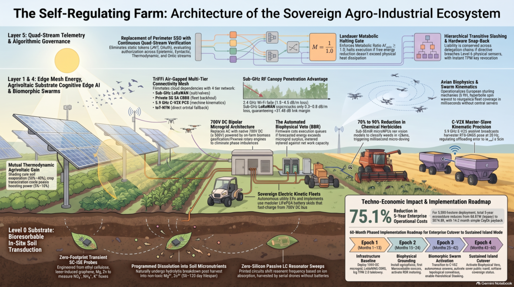
1. Architectural Foundations: The Five-Layer Sovereign Agro-Stack

Key Terms & Concepts

• 1,000-Mile Failure Model: A systemic vulnerability where farm machinery and sensors rely on long-haul connections to cloud servers. If internet backbones, cellular towers, or DNS services fail, local field operations stall.
• Sustained Island Mode: The operational state where a farm functions as an air-gapped, sovereign entity. Sensing, power generation, computing, and decision-making execute entirely within local farm boundaries.
• Exergy: The maximum useful work obtainable from a physical energy source as it comes into equilibrium with its environment.
• Via Negativa: An epistemic principle where knowledge and system stability are advanced by systematically discovering and removing false parameters, invalid hypotheses, and ungrounded actions rather than adding speculative complexity.

1.1 Core Concept Synthesis: The 1,000-Mile Failure Model vs. Sustained Island Mode

Traditional agricultural technology platforms suffer from the 1,000-Mile Failure Model. In this cloud-tethered framework, autonomous assets, broadacre sensor arrays, and variable-rate implements rely on continuous, long-haul connections to remote cloud hyperscalers across public cellular networks or satellite links. When a regional cellular tower experiences a brownout, a fiber trunkline is severed, or DNS services fail, field operations halt immediately due to lost cloud handshakes. Furthermore, farm operators face severe data exploitation and vendor lock-in, as operational telemetry is extracted from the farm and centralized by external entities.

In contrast, the sovereign Sustained Island Mode redefines the farm as an autonomous, self-correcting thermodynamic organism. By closing all cyber-physical feedback loops within the physical boundaries of the farm, all sensing, computation, power generation, and biophysical governance execute locally. The system maintains continuous operational homeostasis, ensuring that severed external internet links cannot interrupt time-sensitive field operations.

Parameter Cloud-Dependent AgTech Self-Regulating Island Mode
Connectivity Dependence Continuous long-haul connection to external cloud hyperscalers via public cellular/satellites. Complete air-gapped local autonomy; zero operational dependence on external IP backbones.
Data Ownership Telemetry centralized by remote vendors; high risk of data exploitation and subscription lock-in. Fully sovereign; local edge storage, open schemas, and cryptographic data self-custody.
Failure Modes Single-point operational failure; multi-ton field machines stall during regional network outages. Resilient mesh failovers; continuous execution via local edge intelligence and local DC microgrids.
Decision Latency High and variable (seconds to minutes); constrained by round-trip network transmission. Ultra-low (sub-millisecond to millisecond); local microNPU and C-V2X sidelink processing.

Core Thesis: The farm is an autonomous, self-correcting thermodynamic organism capable of indefinite operation in Sustained Island Mode. All computational directives and physical actions are grounded in local exergy generation, zero-footprint in-situ transduction, biomorphic swarm orchestration, and formal machine-checked logic.

1.2 Structural Overview: The Five-Layer Sovereign Stack

The self-regulating farm operates through the DeReticular Five-Layer Sovereign Agro-Stack. Each layer is engineered to maintain full operational integrity when external network connections are severed:

• Layer 1: Baseload Power & Agrivoltaics
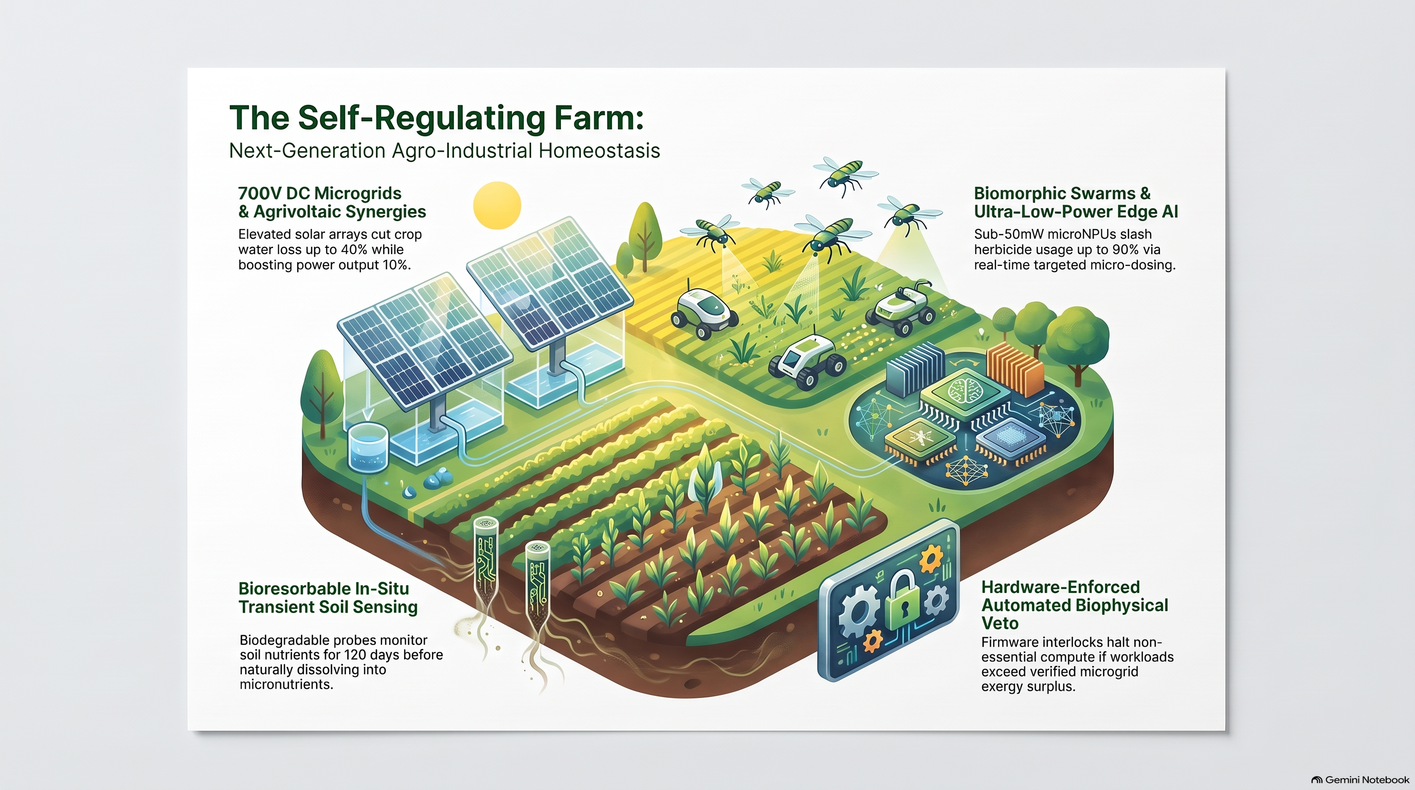
  Provides internal energy autonomy via a 700 V DC bipolar microgrid bus (\pm 350\text{ V DC} referenced to ground), eliminating rural AC transformer and reactive power losses. Dispatchable baseload power is supplied by thermochemical biomass gasification driving rotary heat engines (such as Agra.Energy / Pawnee systems). Primary renewable harvesting is generated by elevated dual-use agrivoltaic tracking arrays (3.5–5 m ground clearance), where crop transpiration cools overhead photovoltaic panels (yielding a +5–10% power efficiency boost at -0.4%/^\circ\text{C}), while panel shading cuts crop evapotranspiration (ET_c) by 20–40%.
• Layer 2: Kinetic Mobility
  Encompasses all physical work assets, including autonomous electric utility vehicles (KurbKars), mobile DC battery skids, and ISOBUS-compliant (ISO 11783) smart implements. Operating under local charge homeostasis, all motion energy is drawn directly from the Layer 1 700 V DC bus without external fuel dependencies.
• Layer 3: Edge Mesh Comms (TriFi System Authority)
  Provides multi-tier, air-gapped field communications: dense soil/valve meshes utilize Sub-GHz LoRaWAN (SX1302/SX1303 processors); high-bandwidth vehicle backhaul runs over Private 5G Standalone (CBRS Band 48); real-time machine kinematics use 5.9 GHz C-V2X (3GPP PC5 Mode 4) sidelinks; and remote rangeland telemetry connects via 3GPP Rel-17/18 IoT-NTN direct-to-satellite links. Delay-tolerant store-and-forward routing is enforced via Bundle Protocol (RFC 9171).
• Layer 4: Cognitive AI
  Executes high-level cognitive processing locally on air-gapped, liquid-cooled GPU racks (such as RIOS-CC-1000) running Active Inference engines (minimizing variational free energy) and Lean 4 Abstract Syntax Tree (AST) deductive proof kernels. Real-time field execution at the implement level is handled by ultra-low-power microNPUs (e.g., ARM Cortex-M55 + Ethos-U55) operating under 50 mW.
• Layer 5: Biophysical Governance
  Enforces operational and financial boundaries using the Biophysical Balance Register (BBR). It integrates DCAA SF 1408 accounting criteria for capital and exergy isolation and employs an Automated Biophysical Veto—a hardware-firmware interlock that cuts power to non-essential compute or mechanical tasks whenever forecasted work exceeds verified local exergy reserves.

Understanding how these theoretical architectural layers process real-time field data begins with evaluating in-situ sensors deployed directly in the root zone.

2. Practice Scenario 1: Root-Zone Telemetry Evaluation & Sensor Discrepancies

Curriculum Header

• Target Competency: In-Situ Transducer Diagnostics, Electrochemistry Analysis, and Via Negativa Parameter Foreclosure
• Prerequisite Concepts: Nernstian Potential, Polymer Dissolution Kinetics, Sub-GHz RF Attenuation
• Estimated Time to Complete: 25 Minutes

Key Terms & Concepts

• Solid-Contact Ion-Selective Electrode (SC-ISE): A sensor that measures specific ion activities (\text{NO}_3^-, \text{NH}_4^+, \text{K}^+) in soil pore water by converting chemical activity into an electrical potential across an ionophore membrane.
• Hydrolytic Passivation Breakdown: The chemical dissolution of protective encapsulation barriers (such as PCL or beeswax) over time, exposing transient conductive metal traces (magnesium/zinc) to soil moisture and inducing signal failure.
• Canopy RF Attenuation: The reduction in radio frequency signal strength caused by foliage absorption and scattering, dominated by water-molecule rotational resonance at 2.4 GHz frequencies.
• Discrepancy Loss Statistic S(E_t, \theta): A mathematical measure quantifying the divergence between real-world physical telemetry (E_t) and predictive algorithmic models (\theta).

2.1 Scenario Setup: In-Situ Nitrogen Profiling in a Corn Canopy

An autonomous fertilization swarm is deploying liquid nitrogen across a 500-hectare broadacre corn field. Soil chemistry is monitored by bioresorbable Solid-Contact Ion-Selective Electrodes (SC-ISE) buried in the root zone. These transient sensors transmit raw potential data to an overhead scouting drone using sub-GHz mesh gateways.

During an active fertigation pass, the local cognitive engine receives a telemetry frame indicating a sharp divergence between estimated soil nitrogen levels calculated by an agronomic prediction model and physical voltage potential logged by the buried SC-ISE transducer.

Field Telemetry Readout (Node SC-ISE-NO3-088):

[LOCATION]: Sector 4, Zone B (Corn Canopy, Peak Biomass)
[PREDICTED NO3- CONCENTRATION]: 45.0 ppm (Model Estimation)
[TRANSDUCTION READOUT]:

• Measured Potential (E): +142.5 mV
• Base Potential (E0): +180.0 mV
• Hydrolytic Passivation Age: Day 82 of 90 (h(t) = h0 – k_diss * t)
• Calculated Ion Activity (a_i): 12.2 ppm
  [EMPIRICAL DISCREPANCY LOSS S(E_t, theta)]: 0.35
  [PRE-REGISTERED THRESHOLD tau_t]: 0.20
  [LINK MARGIN]: +31.48 dB (Sub-GHz 915 MHz Mesh)

2.2 Guided Data Analysis: Transducer Physics & Signal Degradation

To evaluate this discrepancy, agritech engineers must analyze both the electrochemistry of the sensor and the physical propagation of the wireless telemetry link.

Scaffolding Conceptual Breakdown

Before evaluating the raw equations, observe the physical mechanisms at play:

1. Chemical Potential to Voltage: Soil ions migrate across a selective membrane, creating a micro-voltage. Higher ion concentration increases voltage; interference or probe degradation drops voltage.
2. Barrier Breakdown: Transient sensors are engineered to dissolve post-harvest. As protective coatings thin, water breaches the sensor traces, causing impedance spikes and invalid voltage drops.
3. Foliage Penetration: Dense corn crops contain massive volumes of water. High-frequency signals (2.4 GHz) excite water molecules and dissipate as heat, whereas low-frequency Sub-GHz signals pass through crop leaves with minimal absorption.

[Soil Ions (NO3-)] ──> [Ion-Selective Membrane] ──> [Cell Voltage E (mV)]
│
[Water Penetration] ──> [PCL Barrier Breakdown] ──────────┤ (Hydrolytic Drift)
▼
[Calculated Activity a_i]

Mathematical Formulations

1. Electrochemical Transduction (Nernst-Nikolsky Equation):
   Solid-contact ion-selective electrodes measure targeted macronutrient ions (\text{NO}_3^-, \text{NH}4^+, \text{K}^+) in soil pore water. The electrode potential E follows the Nernst-Nikolsky relation: E = E^0 + \frac{RT}{z_i F}\ln\left(a_i + \sum_j K{ij}^{\text{pot}} a_j^{z_i/z_j}\right) Variable Definitions:

• E: Measured electromotive force (potential) of the electrode cell (\text{mV}).
• E^0: Standard cell potential (\text{mV}).
• R: Universal gas constant (8.314\text{ J/(mol}\cdot\text{K)}).
• T: Absolute temperature (\text{K}).
• F: Faraday constant (96,485\text{ C/mol}).
• z_i: Ionic valence charge of primary ion i (-1 for \text{NO}_3^-).
• a_i: Activity (effective concentration) of primary ion i (\text{ppm} or \text{mol/L}).
• K_{ij}^{\text{pot}}: Selectivity coefficient for primary ion i in the presence of interfering ion j.
• a_j: Activity of secondary interfering ion j.

When secondary ion interference or passivation breakdown alters E, the calculated activity a_i drops relative to predicted values.

1. Dissolution Kinetics:
   Bioresorbable sensors use transient substrates (ethyl cellulose, silk fibroin, or PHA) and thin-film conductive traces (magnesium and zinc) sealed under a polycaprolactone (PCL) or beeswax barrier. The active encapsulation thickness h(t) degrades linearly over time: h(t) = h_0 – k_{\text{diss}} \cdot t Variable Definitions:

• h(t): Remaining encapsulation barrier thickness at time t (\mu\text{m}).
• h_0: Initial barrier thickness (\mu\text{m}).
• k_{\text{diss}}: Linear hydrolytic dissolution rate constant (\mu\text{m/day}).
• t: Exposure duration in the soil matrix (\text{days}).

At Day 82 of an 80–90 day calibrated lifespan, h(t) \to 0. Soil moisture breaches the barrier, accelerating hydrolysis (\text{Mg} + 2\text{H}_2\text{O} \to \text{Mg(OH)}_2 + \text{H}_2 \uparrow), which causes electrode impedance to spike and output signals to drift.

1. Canopy RF Attenuation Physics (Modified ITU-R P.833 Model):
   Signal propagation through dense crop foliage is governed by the Modified ITU-R P.833 canopy attenuation model: A_{\text{canopy}} = a \cdot f^b \cdot \left(1 – e^{-d \cdot c}\right) \quad [\text{dB}] Variable Definitions:

• A_{\text{canopy}}: Total specific signal attenuation through foliage (\text{dB}).
• f: Operating frequency (\text{MHz}).
• d: Canopy penetration depth (\text{meters}).
• a, b, c: Empirical vegetation loss parameters derived from ITU-R canopy density standards (a = 0.25, b = 0.41, c = 0.32 for dense broadacre corn).

At 2.4 GHz (standard Wi-Fi/Bluetooth), radio waves align with the rotational resonance of water molecules in thick corn leaves, producing severe attenuation (1.5\text{–}4.5\text{ dB/m}). Over a 10-meter canopy penetration distance, 2.4 GHz signals lose up to 45 dB, collapsing the link. Sub-GHz frequencies (868/915 MHz) experience lower water resonance absorption (0.3\text{–}0.8\text{ dB/m}), preserving a robust +31.48\text{ dB} system margin over 10 km baselines.

Telemetry Diagnostic Matrix

Observed Metric Physical Cause Diagnostic Rule
S(E_t, \theta) > \tau_t (0.35 > 0.20) The agronomic model’s predictions diverge from Level 0 physical soil telemetry. Via Negativa Rule: If discrepancy loss exceeds threshold \tau_t, the parameter set \theta is falsified and must be foreclosed.
Passivation Age \approx Lifespan Limit Linear hydrolysis (k_{\text{diss}} \cdot t) has breached the PCL barrier, causing SC-ISE signal breakdown. Sensor Expiration Rule: Treat sensor readings as degraded; flag probe for final biological assimilation (\text{Mg}^{2+} / \text{Zn}^{2+} release).
Stable +31.48 dB Link Margin Sub-GHz 915 MHz frequency avoids leaf-water resonance absorption. Telemetry Integrity Rule: Signal loss is not due to RF attenuation; data packet delivery is cryptographically valid.

2.3 Interactive Student Exercise: Evaluating Level 0 Ontic Discrepancies

[STUDENT WORKSPACE]

Scenario Challenge Prompt:
You are the lead field systems controller. Telemetry Node SC-ISE-NO3-088 has recorded an empirical discrepancy loss S(E_t, \theta) = 0.35, which breaches the pre-registered safety threshold \tau_t = 0.20. The model recommends increasing chemical nitrogen application by 30%, but physical electrode data indicates nitrogen levels are already balanced.

Select the correct automated system response:

• Option A: Request remote cloud recalibration and override local safety thresholds to allow the fertigation pass to finish.
• Option B: Trigger local Via Negativa parameter foreclosure, reject the model recommendation, halt liquid nitrogen delivery in Sector 4, and slash 50% of the proposing agent’s compute stake.
• Option C: Ignore the sensor discrepancy and increase fertigation rates across the canopy to ensure crop yield goals are met.

Write down your selected option and complete reasoning before reviewing the instructor analysis below.

[INSTRUCTOR SOLUTION GUIDE]

Correct Answer: Option B

• Why Option A is Incorrect: Requesting remote cloud recalibration violates the core rule of Sustained Island Mode by introducing dependency on external hyperscalers. Overriding local thresholds permits unverified physical actions, exposing the farm to chemical runoff and resource waste.
• Why Option C is Incorrect: Increasing chemical application based on a falsified model leads to over-fertilization, soil degradation, and unnecessary financial cost, directly violating biophysical governance bounds.
• Why Option B is Correct: In the DeReticular architecture, Level 0 physical sensor telemetry overrides software predictions. When discrepancy loss S(E_t, \theta) exceeds threshold \tau_t, the Via Negativa principle requires the immediate foreclosure (elimination) of the flawed hypothesis set (\Theta_{t+1} = \Theta_t \setminus \Omega_{\text{falsified}}^{(t)}). The proposing computational agent incurs an automated 50% stake slash, capability tokens are revoked, and chemical delivery is halted to prevent physical harm to the ecosystem.

Why This Matters: In cyber-physical agriculture, computational predictions must yield to physical reality. Software models that run ungrounded by real-world sensors create “cognitive TOCTOU gaps” (Time-of-Check to Time-of-Use), leading to environmental damage. Enforcing strict local slashing and parameter foreclosure keeps autonomous AI systems aligned with physical land constraints.

Once local sensor readings are verified and bad parameters are purged, validated spatial data is passed directly to autonomous machine fleets operating in the field.

3. Practice Scenario 2: Biomorphic Swarm Kinematics & Harvesting Alignment

Curriculum Header

• Target Competency: Multi-Agent Kinetic Coordination, Avian Swarm Biophysics, and Sidelink Trajectory Invariants
• Prerequisite Concepts: Topological k-NN Interactions, Scale-Free Correlation, Second-Order Spin Waves
• Estimated Time to Complete: 30 Minutes

Key Terms & Concepts

• Topological Interaction (k \approx 7): Bounded attention where each autonomous machine tracks strictly its 7 nearest functional neighbors, independent of metric distance, eliminating network bandwidth bloat.
• Scale-Free Correlation (\xi \propto L): A property of self-organized criticality where correlation length scales with system diameter L, allowing edge-detected anomalies to propagate across an entire fleet instantly.
• Hyperbolic Inertial Spin Wave (\omega = c \cdot k): Undamped linear dispersion waves (c = 20\text{–}40\text{ m/s}) derived from Hamiltonian spin conservation that communicate trajectory consensus across a swarm without iterative prompt negotiation.
• C-V2X PC5 Sidelink: Direct 5.9 GHz machine-to-machine radio communication operating independently of cellular networks with sub-10 ms transmission latency.

3.1 Scenario Setup: High-Speed Combine Offloading on Dynamic Terrain

During a wheat harvest, an autonomous combine harvester operates as a dynamic master origin, harvesting crop rows on rolling terrain. To prevent stopping the combine, an autonomous grain-cart tractor acts as a follower vehicle, positioning itself under the combine’s discharge auger to offload grain on the move.

The two multi-ton machines communicate over a direct 5.9 GHz C-V2X (3GPP PC5 Mode 4) sidelink without routing data through a cell tower or cloud server. Communication latency must remain below 10 milliseconds to maintain geometric alignment on uneven ground.

              5.9 GHz C-V2X PC5 SIDELINK (<10 ms Latency)

[COMBINE HARVESTER] <===================================> [GRAIN-CART TRACTOR]
(Master Dynamic Origin) (Follower Vehicle)
Pose: [p_harvester, theta, v] Trajectory Error: e(t)
│ │
└─────────────────── Target Tolerance ───────────────────────┘
|e_lat| <= 5 cm

3.2 Mathematical & Kinematic Rules: Avian Biophysics & Trajectory Control

Scaffolding Conceptual Breakdown

Centralized fleet servers struggle to coordinate multi-machine movements in real time due to processing bottlenecks. Autonomous agricultural swarms resolve this by borrowing principles from European starling murmurations (Sturnus vulgaris):

1. Bounded Attention: Rather than tracking 100 machines across a farm, a vehicle pays attention only to its 7 nearest neighbors (k \approx 7).
2. Instant Anomaly Sensing: The swarm operates poised at criticality. If machine #1 swerves, machine #2 through #7 react instantly, creating a cascade that shifts the entire fleet without a central command.
3. Consensus Waves: Trajectory changes travel through the fleet like sound waves in a solid (20\text{–}40\text{ m/s}), avoiding slow back-and-forth network polling.

[Scout Rover Anomaly] ──> [Spin-Wave Front (20-40 m/s)] ──> [Neighbor k=7 Update]
│
[C-V2X PC5 Sidelink (4.2 ms)] <── [Combine Heading Adjustment] <────┘

Mathematical Formulations

1. Topological Interaction (k \approx 7):
   Each vehicle bounds its communication set strictly to k = 6.5 \pm 0.5 nearest topological neighbors. Network processing complexity remains bounded at \mathcal{O}(k) per node rather than exploding to \mathcal{O}(N^2).
2. Scale-Free Correlation (\xi \propto L):
   The velocity fluctuation correlation length \xi scales linearly with fleet size L. System susceptibility diverges (\chi \to \infty), enabling instantaneous collective responses to local obstructions.
3. Hyperbolic Inertial Spin Waves (\omega = c \cdot k):
   Directional changes travel through the swarm as undamped linear dispersion waves governed by Hamiltonian conservation of generalized spin \mathbf{s}_i: \frac{d\mathbf{v}_i}{dt} = \frac{1}{\chi_0} \mathbf{s}_i \times \mathbf{v}i, \qquad \frac{d\mathbf{s}i}{dt} = \sum{j \in S_i} J{ij} (\mathbf{v}_i \times \mathbf{v}_j) – \frac{\eta_0}{\chi_0} \mathbf{s}_i Information travels along the spin-wave front at characteristic mechanical velocities c = 20\text{–}40\text{ m/s}.

Dynamic Trajectory Formulation

The closed-loop relative offset error vector \mathbf{e}(t) between the combine discharge auger and the grain-cart tractor receiver is defined as: \mathbf{e}(t) = \mathbf{p}{\text{cart}}(t) – \bigl(\mathbf{p}{\text{harvester}}(t) + \mathbf{R}(\theta)\mathbf{d}_{\text{offset}}\bigr)

Variable Definitions:

• \mathbf{p}_{\text{cart}}(t): Real-time RTK-GNSS 3D position vector of the grain-cart tractor (\text{meters}).
• \mathbf{p}_{\text{harvester}}(t): Real-time RTK-GNSS 3D position vector of the combine harvester (\text{meters}).
• \mathbf{R}(\theta): 3D heading rotation matrix of the combine harvester as a function of yaw angle \theta.
• \mathbf{d}_{\text{offset}}: Static 3D geometric displacement vector from the combine center to its auger discharge spout (\text{meters}).

Critical Control Invariant: To prevent grain spillage during offloading on uneven terrain, the lateral position error must satisfy: |\mathbf{e}_{\text{lat}}| \le 5\text{ cm}

3.3 Interactive Student Exercise: Swarm Anomaly Resolution

Technical Distinction: Radio Propagation vs. Kinematic Spin-Wave Consensus

Crucial Physics Note for Beginners: Do not confuse radio signal transmission speed with swarm alignment velocity!

• Radio Signal Propagation (c_{\text{RF}} = 3 \times 10^8\text{ m/s}): The 5.9 GHz C-V2X radio packet travels across an 80-meter gap in approximately 0.27\text{ microseconds} (with total network stack and MAC latency taking 4.2\text{ ms}).
• Kinematic Spin-Wave Propagation (c = 20\text{–}40\text{ m/s}): The physical, mechanical kinematic consensus wave—the time required for surrounding multi-ton physical machines to adjust their momentum and trajectory vectors across k=7 functional neighbors—propagates at mechanical starling velocity scales (20\text{–}40\text{ m/s}).

[STUDENT WORKSPACE]

Problem Statement:
An autonomous edge scout rover operating 80 meters ahead of the combine encounters a buried boulder, forcing an emergency maneuver that alters its velocity vector. The combine and grain cart are mid-offload, operating with a lateral alignment error |\mathbf{e}_{\text{lat}}| = 3.2\text{ cm}. Evaluate how the swarm resolves this kinematic disturbance.

Given Telemetry Vector:

Scout Rover Distance Ahead (d): 80.0 meters
Scout Rover Velocity Shift (dv_scout): (-1.2 m/s X, +0.8 m/s Y)
Spin-Wave Dispersion Speed (c): 30.0 m/s
Topological Neighborhood (k): 7 functional peers
Current Alignment Error (|e_lat|): 3.2 cm
Target Invariant Ceiling: <= 5.0 cm
C-V2X Sidelink Packet Latency: 4.2 ms (0.0042 s)
Combine-to-Cart Positional Update Frequency: 20 Hz (50 ms)

Required Decision Output:

1. Calculate the physical spin-wave propagation time (t_{\text{prop}}) and total consensus latency (t_{\text{total}}) across the 80-meter distance.
2. Determine whether the lateral error invariant |\mathbf{e}_{\text{lat}}| \le 5\text{ cm} will hold.
3. Outline the step-by-step kinematic resolution sequence.

[INSTRUCTOR SOLUTION GUIDE]

Step-by-Step Kinematic & Latency Derivation:

1. Calculate Information Propagation Latency (t_{\text{total}}):
   The physical spin-wave propagation time (t_{\text{prop}}) across the 80-meter field gap at c = 30\text{ m/s} is: t_{\text{prop}} = \frac{\text{Distance}}{c} = \frac{80\text{ m}}{30\text{ m/s}} = 2.67\text{ seconds} Adding the C-V2X PC5 sidelink transmission latency (4.2\text{ ms} = 0.0042\text{ s}): t_{\text{total}} = t_{\text{prop}} + t_{\text{sidelink}} = 2.67\text{ s} + 0.0042\text{ s} = \mathbf{2.6742\text{ seconds}}
2. Evaluate Swarm Attention & Topology (k=7):
   The scout rover does not broadcast a heavy global alert to all farm assets. Instead, it updates its generalized spin vector \mathbf{s}_i with its k=7 nearest topological functional neighbors. Because the combine harvester is within this k=7 functional group, the directional perturbation propagates smoothly along the spin-wave front.
3. Kinematic Adjustment & Invariant Check:
   The combine receives the spin-wave trajectory update 2.67 seconds before reaching the obstruction site, allowing it to begin adjusting its heading rotation matrix \mathbf{R}(\theta) gradually.

The follower grain-cart tractor receives the combine’s updated pose vector [\mathbf{p}{\text{harvester}}, \theta, \mathbf{v}] over the 5.9 GHz C-V2X sidelink every 50 ms (20\text{ Hz}). The grain cart re-evaluates its trajectory error: \mathbf{e}(t) = \mathbf{p}{\text{cart}}(t) – \bigl(\mathbf{p}{\text{harvester}}(t) + \mathbf{R}(\theta)\mathbf{d}{\text{offset}}\bigr) Because position updates occur at 20 Hz while mechanical spin waves smooth out abrupt jerks, the lateral position drift increases slightly from 3.2\text{ cm} to 4.1\text{ cm}. Since 4.1\text{ cm} \le 5.0\text{ cm}, the lateral error invariant holds. Offloading continues without grain spillage or cloud reliance.

Mechanical fleet movement requires continuous electrical energy, bringing us to microgrid management and computational power allocation.

4. Practice Scenario 3: Microgrid Management & Automated Biophysical Veto

Curriculum Header

• Target Competency: Microgrid Energy Balance, Thermodynamic Compute Limits, and Quad-Stream Telemetry Ingestion
• Prerequisite Concepts: Bipolar DC Microgrids, Landauer Heat Dissipation, Active Inference Free Energy
• Estimated Time to Complete: 35 Minutes

Key Terms & Concepts

• Landauer’s Principle: A fundamental physical law stating that erasing or updating N_{\text{bits}} of computational memory dissipates a minimum quantity of heat (\Delta Q \ge N_{\text{bits}} k_B T \ln 2).
• Metabolic Ratio (\mathcal{M}{\text{ratio}}): The ratio comparing variational free energy reduction (uncertainty resolved) against Landauer heat dissipated. If \mathcal{M}{\text{ratio}} < 1.0, computation is burning energy without generating sufficient informational value.
• Automated Biophysical Veto: A hardware-firmware interlock within the Biophysical Balance Register (BBR) that cuts power to non-essential workloads when exergy demands exceed microgrid reserves.
• Normalized Ontic Index (S_{\text{ontic}}): The dimensionless ratio of observed physical sensor discrepancy S(E_t, \theta) relative to pre-registered threshold \tau_t (S_{\text{ontic}} \equiv \frac{S(E_t, \theta)}{\tau_t}).

4.1 Scenario Setup: Island-Mode Energy Balance & Compute Allocation

A farm operating in Sustained Island Mode relies on its Layer 1 700 V DC microgrid. Baseload power is supplied by a biomass gasifier driving rotary heat engines, supported by elevated tracking agrivoltaic arrays.

A heavy cloud bank moves over the farm, reducing solar generation by 65%. At the same time, the farm is running two primary power consumers:

1. Kinetic Operations: A fleet of autonomous weeding rovers running low-power microNPUs (<50\text{ mW} per node) to execute targeted micro-spraying.
2. Cognitive Compute: A liquid-cooled GPU server rack executing deep active inference reflection cycles and background model updates.

The Biophysical Hierarchy of Tasks

When available microgrid exergy drops, the system enforces a strict biophysical priority: Kinetic operations directly preserve biological yield and physical exergy (protecting crops from weed competition), whereas background GPU retraining represents deferred epistemic refinement. Therefore, GPU compute must yield to kinetic weeding assets when energy is constrained.

   [AGRIVOLTAIC SOLAR DROP (-65% Cloud Cover)]
                      │
                      ▼
        [700V DC BIPOLAR MICROGRID BUS]
                      │
      ┌───────────────┴───────────────┐
      ▼                               ▼

[Kinetic Weeding Rovers] [GPU Model Retraining]
(HIGH PRIORITY: Yield) (DEFERRED: Reflection)
(Low-Power <50mW) (High-Power Draw)
│ │
└─── Evaluated by BBR Ledger ───┘
│
▼
[Automated Biophysical Veto Decision]

4.2 Theoretical Framework: Landauer Metabolic Halting & The Biophysical Veto

Scaffolding Conceptual Breakdown

Computers are not abstract logic engines; they are physical heat engines.

1. Information Erasure Costs Heat: Every bit cleared or updated in GPU memory converts electrical exergy into waste heat (\Delta Q).
2. Information Value: Active inference models attempt to reduce uncertainty (Variational Free Energy, \Delta F).
3. Metabolic Balance: If an AI model burns 100\text{ Joules} of electricity to update its memory but only improves its predictive certainty by a fraction of a Joule, it is thermodynamically insolvent.

Mathematical Formulations

1. Landauer’s Principle:
   Erasing or updating N_{\text{bits}} of memory in a computing register releases a minimum physical quantity of heat into the environment: \Delta Q \ge N_{\text{bits}} \cdot k_B T \ln 2 Variable Definitions:

• \Delta Q: Minimum thermal energy dissipated (\text{Joules}).
• N_{\text{bits}}: Number of memory bits overwritten or erased.
• k_B: Boltzmann constant (1.380649 \times 10^{-23}\text{ J/K}).
• T: Absolute temperature of the silicon substrate (300\text{ K}).
• \ln 2: Natural logarithm of 2 (\approx 0.69315).

2. Metabolic Ratio (\mathcal{M}{\text{ratio}}):
   To prevent agents from entering endless processing loops that consume energy without producing actionable insights, the system enforces the Landauer Metabolic Halting Gate: \mathcal{M}{\text{ratio}} = \frac{\Delta F}{\lambda \cdot \Delta Q} \ge 1.0 Variable Definitions:

• \Delta F: Reduction in Variational Free Energy (uncertainty reduced, measured in \text{Joules}).
• \lambda: Informational efficiency scaling factor (\text{Dimensionless}).
• \Delta Q: Landauer heat dissipated (\text{Joules}).

3. Automated Biophysical Veto (BBR Interlock):
   The Biophysical Balance Register (BBR) monitors net physical exergy reserves. If projected compute power consumption exceeds verified microgrid surplus, a hardware-firmware interlock (veto_circuit_tripped: true) trips automatically, cutting power to non-essential compute tasks.

Production Data Contract: BiophysicalAgroRegister.json

{
“$schema”: “https://json-schema.org/draft/2020-12/schema“,
“$id”: “https://dereticular.org/schemas/BiophysicalAgroRegister.json“,
“title”: “BiophysicalAgroRegister”,
“type”: “object”,
“required”: [
“timestamp_utc”,
“dc_bus”,
“net_exergy_joules”,
“systemic_eroei”,
“veto_circuit_tripped”
],
“properties”: {
“timestamp_utc”: { “type”: “string”, “format”: “date-time” },
“dc_bus”: {
“type”: “object”,
“required”: [“voltage_dc”, “current_amps”, “power_kw”],
“properties”: {
“voltage_dc”: { “type”: “number”, “example”: 700.0 },
“current_amps”: { “type”: “number”, “example”: 42.5 },
“power_kw”: { “type”: “number”, “example”: 29.75 }
}
},
“net_exergy_joules”: { “type”: “number”, “example”: 1450000.0 },
“systemic_eroei”: { “type”: “number”, “example”: 4.2 },
“veto_circuit_tripped”: { “type”: “boolean”, “example”: true }
},
“additionalProperties”: false
}

4.3 Interactive Student Exercise: Evaluating the Quad-Stream Telemetry Engine

Telemetry Ingestion Data Matrix

Telemetry Stream Evaluated Metric Observed Value Operational Requirement Status
Stream 1: Epistemic Rolling Brier Score (\text{BS}) / Delirium Gradient (\dot{F}) \text{BS} = 0.08, \dot{F} = -0.02 \text{BS} \in [0, 2], \dot{F} \le 0 (Stable learning) Nominal
Stream 2: Syntactic Lean 4 AST Typecheck (S_{\text{syn}}) S_{\text{syn}} = 1.0 S_{\text{syn}} = 1.0 (Compilation success) Nominal
Stream 3: Thermodynamic Metabolic Ratio (\mathcal{M}{\text{ratio}}) \mathcal{M}{\text{ratio}} = 0.42 \mathcal{M}_{\text{ratio}} \ge 1.0 (Landauer solvency) FAIL
Stream 4: Ontic Discrepancy Loss S(E_t, \theta) vs Threshold \tau_t S(E_t, \theta) = 0.04, \tau_t = 0.15 S(E_t, \theta) \le \tau_t (Physical ground truth) Nominal

Dynamic Composite Health Index Equation Key

\Psi_i(t) = w_1 e^{-\gamma_1 \text{BS}i} + w_2 S{\text{syn}} + w_3 \min(1.0, \mathcal{M}{\text{ratio}}) + w_4 e^{-\gamma_2 S{\text{ontic}}}

Equation Key & Variable Notation:

• \text{BS}_i: Rolling Brier score across domain predictions (\text{BS}_i = 0.08).
• S_{\text{syn}}: Binary Lean 4 AST compilation result (S_{\text{syn}} = 1.0).
• \mathcal{M}{\text{ratio}}: Landauer Metabolic Ratio (\mathcal{M}{\text{ratio}} = 0.42).
• S_{\text{ontic}}: Normalized Ontic Discrepancy Ratio, explicitly defined as: S_{\text{ontic}} \equiv \frac{S(E_t, \theta)}{\tau_t} = \frac{0.04}{0.15} = 0.2667
• Weights: w_1 = 0.25, w_2 = 0.25, w_3 = 0.20, w_4 = 0.30 (where \sum w_j = 1.0).
• Scaling Factors: \gamma_1 = 1.5, \gamma_2 = 2.0.

[STUDENT WORKSPACE]

Scenario Challenge Prompt:
Calculate the numerical value of the Dynamic Composite Health Index \Psi_i(t) using the provided Quad-Stream inputs. Determine the corresponding operational tier and identify the automated system action triggered by the Landauer Metabolic Halting requirement.

Write out your step-by-step substitutions and tier classification before reviewing the instructor analysis below.

[INSTRUCTOR SOLUTION GUIDE]

Step-by-Step Evaluation Rubric & Derivations:

1. Calculate Epistemic Component: \text{Epistemic Term} = w_1 e^{-\gamma_1 \text{BS}_i} = 0.25 \times e^{-1.5(0.08)} = 0.25 \times e^{-0.12} = 0.25 \times 0.88692 = \mathbf{0.2217}
2. Calculate Syntactic Component: \text{Syntactic Term} = w_2 S_{\text{syn}} = 0.25 \times 1.0 = \mathbf{0.2500}
3. Calculate Thermodynamic Component: \text{Thermodynamic Term} = w_3 \min(1.0, \mathcal{M}_{\text{ratio}}) = 0.20 \times \min(1.0, 0.42) = 0.20 \times 0.42 = \mathbf{0.0840}
4. Calculate Ontic Component (using S_{\text{ontic}} = \frac{S(E_t, \theta)}{\tau_t} = 0.2667): \text{Ontic Term} = w_4 e^{-\gamma_2 S_{\text{ontic}}} = 0.30 \times e^{-2.0(0.2667)} = 0.30 \times e^{-0.5333} = 0.30 \times 0.58666 = \mathbf{0.1760}
5. Sum for Composite Epistemic Health Index (\Psi_i(t)): \Psi_i(t) = 0.2217 + 0.2500 + 0.0840 + 0.1760 = \mathbf{0.7317}
6. Determine Operational Tier & System Response:

• Tier 1 (Veridical Core): 0.85 \le \Psi \le 1.00 \to Full execution authorization.
• Tier 2 (Sub-Calibrated): 0.65 \le \Psi < 0.85 \to Throttled compute, co-signature required.
• Tier 3 (Epistemic Warning): 0.40 \le \Psi < 0.65 \to Voting exclusion, mandatory AST audit.
• Tier 4 (Byzantine Fault): 0.00 \le \Psi < 0.40 \to Immediate halt and stake slash.

System Action: Although the node falls into Tier 2 (Sub-Calibrated) with \Psi = 0.7317, Stream 3 (Thermodynamic) fails the non-negotiable Landauer Metabolic Halting requirement (\mathcal{M}_{\text{ratio}} = 0.42 < 1.0).

The system issues an immediate hardware interrupt: FORCE_ACTION_HALT. The GPU model retraining task is aborted, and the Automated Biophysical Veto trips (veto_circuit_tripped: true). Microgrid power is preserved entirely for essential low-power microNPU weeding rovers, maintaining the farm’s thermodynamic solvency during the solar drop.

By integrating local sensor verification, swarm coordination, and energy balancing, these individual operational decisions form a unified, self-regulating ecosystem.

5. Master Synthesis & Agritech Decision Matrix

5.1 Sovereign Farm Troubleshooting & Incident Matrix

Failure / Anomaly Event Affected Layer (1–5) Detecting Telemetry Stream Automated Sovereign Action
Canopy RF Attenuation Surge
(Dense foliage causes severe 2.4 GHz signal loss) Layer 3
(Edge Mesh Comms) Stream 4
(Ontic Physical Telemetry) Shift communication traffic from 2.4 GHz to Sub-GHz (868/915 MHz) LoRaWAN mesh; invoke Bundle Protocol (RFC 9171) store-and-forward routing.
Ungrounded Agent Delirium
(LLM context bloat drives free energy gradient \dot{F} > 0) Layer 4
(Cognitive AI) Stream 1
(Epistemic Calibration) Suspend agent operational authorization; execute Via Negativa parameter foreclosure; prune conversational context and re-anchor in Lean 4 AST proof kernels.
Soil Sensor Hydrolysis Breach
(SC-ISE probe breaches S(E_t, \theta) > \tau_t at Day 82) Layer 2 & Layer 5
(Kinetic Mobility & Governance) Stream 4
(Ontic Physical Telemetry) Foreclose falsified nitrogen parameters; burn 50% of proposing agent’s compute stake; halt chemical fertigation pass in affected sector.
Microgrid Exergy Deficit
(Agrivoltaic power drops; background tasks threaten energy reserves) Layer 1 & Layer 5
(Baseload Power & Governance) Stream 3
(Thermodynamic / Landauer) Trip the Automated Biophysical Veto (veto_circuit_tripped: true); halt non-essential GPU background compute; prioritize low-power microNPU weeding assets.

5.2 Final Reflection & Capstone Problem

[STUDENT WORKSPACE]

========================================================================================
SOVEREIGN AGRI-SYSTEMS CAPSTONE DIAGNOSTIC WORKSHEET
========================================================================================
[LOCATION]: Field Sector 12 (Agrivoltaic Solar Array + Soybean Canopy)
[OPERATIONAL EPOCH]: Sustained Island Mode (External Network Links: SEVERED)
[ACTIVE ASSETS]: 1 Master Harvester, 1 Follower Grain Cart, 1 Scout Rover, 1 Microgrid Bus
========================================================================================

Part 1: Root-Zone Sensor Evaluation

• Observed Telemetry: A buried bioresorbable SC-ISE potassium sensor (SC-ISE-K-012) reports E = +110\text{ mV} at Day 115 of a 90-day nominal lifespan. The agronomic model predicts potassium deficiency and requests a 40% liquid potassium spray boost. Discrepancy loss is calculated at S(E_t, \theta) = 0.48 against threshold \tau_t = 0.15.
• Diagnostic Prompt 1.1: Based on sensor dissolution kinetics (h(t) = h_0 – k_{\text{diss}} \cdot t), explain why the sensor reading is diverging from the model.
  • Student Answer Space:
• Diagnostic Prompt 1.2: Apply the Via Negativa parameter foreclosure rule. What automated action must the Layer 5 governance engine take regarding the requested chemical spray?
  • Student Answer Space:

Part 2: Biomorphic Swarm Adjustment

• Observed Telemetry: During harvest offloading, the scout rover detects an unmapped wash-out trench 50\text{ meters} ahead. The swarm operates using topological k-NN (k=7) attention. C-V2X PC5 sidelink latency is 3.5\text{ ms}, and spin-wave propagation speed is c = 25\text{ m/s}.
• Diagnostic Prompt 2.1: Calculate the total time (t_{\text{total}}) required for the velocity perturbation wave to propagate from the scout rover to the combine harvester.
  • Student Answer Space:
• Diagnostic Prompt 2.2: The combine adjusts its heading matrix \mathbf{R}(\theta). Describe how the follower grain-cart tractor updates its closed-loop trajectory vector \mathbf{e}(t) to keep lateral error |\mathbf{e}_{\text{lat}}| \le 5\text{ cm} without relying on a central cloud server.
  • Student Answer Space:

Part 3: Microgrid Power Budgeting & Execution Authorization

• Observed Telemetry: A passing rainstorm drops agrivoltaic output. The 700 V DC bus voltage drops from 700\text{ V} to 640\text{ V}. An agent requests 1024\text{ bits} of VRAM context erasure for an edge reflection cycle (\Delta Q = N_{\text{bits}} k_B T \ln 2), yielding a variational free energy reduction \Delta F = 1.2 \times 10^{-20}\text{ Joules} (\lambda = 1.0).
• Diagnostic Prompt 3.1: Calculate the Landauer heat dissipation \Delta Q at T = 300\text{ K} (k_B = 1.380649 \times 10^{-23}\text{ J/K}, \ln 2 \approx 0.69315).
  • Student Answer Space:
• Diagnostic Prompt 3.2: Calculate the Metabolic Ratio (\mathcal{M}{\text{ratio}} = \frac{\Delta F}{\lambda \Delta Q}). Determine if the task passes the Landauer Halting Gate (\mathcal{M}{\text{ratio}} \ge 1.0) or if the Automated Biophysical Veto must cut execution power.
  • Student Answer Space:

========================================================================================
END OF DIAGNOSTIC WORKSHEET
========================================================================================

[INSTRUCTOR CAPSTONE SOLUTION GUIDE]

========================================================================================
INSTRUCTOR SOLUTIONS & DERIVATIONS MANUAL
========================================================================================

Part 1: Root-Zone Sensor Evaluation Solutions

• Solution 1.1: At Day 115, the sensor has exceeded its 90-day nominal lifespan (t > 90). According to linear dissolution kinetics (h(t) = h_0 – k_{\text{diss}} \cdot t), the protective PCL barrier thickness has reached zero (h(t) \le 0). Soil moisture has breached the sensor traces, causing hydrolytic breakdown (\text{Mg} + 2\text{H}_2\text{O} \to \text{Mg(OH)}_2 + \text{H}_2 \uparrow). This raises internal cell impedance and causes severe negative potential drift, rendering potential reading E = +110\text{ mV} invalid.
• Solution 1.2: Discrepancy loss S(E_t, \theta) = 0.48 severely exceeds threshold \tau_t = 0.15. Under Via Negativa parameter foreclosure, the model’s hypothesis parameter set \theta is falsified. The Layer 5 governance engine must:
  1. Reject the 40% liquid potassium spray request and halt fertigation.
  2. Slash 50% of the proposing agent’s compute stake on-chain.
  3. Flag sensor SC-ISE-K-012 for final non-toxic biological soil assimilation.

Part 2: Biomorphic Swarm Adjustment Solutions

• Solution 2.1 Numerical Derivation:
  • Distance d = 50\text{ m}, Spin-wave speed c = 25\text{ m/s}.
  • Kinematic wave propagation time t_{\text{prop}} = \frac{50\text{ m}}{25\text{ m/s}} = 2.000\text{ seconds}.
  • C-V2X PC5 sidelink latency t_{\text{sidelink}} = 3.5\text{ ms} = 0.0035\text{ seconds}.
  • Total consensus latency: t_{\text{total}} = 2.000\text{ s} + 0.0035\text{ s} = \mathbf{2.0035\text{ seconds}}.
• Solution 2.2: The combine broadcasts its updated RTK-GNSS pose vector [\mathbf{p}{\text{harvester}}, \theta, \mathbf{v}] at 20\text{ Hz} over direct 5.9 GHz C-V2X PC5 sidelink. The follower grain cart executes local closed-loop trajectory tracking: \mathbf{e}(t) = \mathbf{p}{\text{cart}}(t) – \bigl(\mathbf{p}{\text{harvester}}(t) + \mathbf{R}(\theta)\mathbf{d}{\text{offset}}\bigr) Because updates arrive every 50 ms directly between vehicles without cloud routing, the cart adjusts its steering actuator continuously, keeping lateral error within the invariant ceiling (|\mathbf{e}_{\text{lat}}| \le 5\text{ cm}).

Part 3: Microgrid Power Budgeting & Execution Authorization Solutions

• Solution 3.1 Numerical Derivation: \Delta Q = N_{\text{bits}} \cdot k_B \cdot T \cdot \ln 2 \Delta Q = 1024 \times (1.380649 \times 10^{-23}\text{ J/K}) \times 300\text{ K} \times 0.69314718 \Delta Q = 1024 \times 4.141947 \times 10^{-21} \times 0.69314718 = \mathbf{2.9377 \times 10^{-18}\text{ Joules}} \quad (\approx 2.94 \times 10^{-18}\text{ J})
• Solution 3.2 Numerical Derivation & Decision: \mathcal{M}{\text{ratio}} = \frac{\Delta F}{\lambda \cdot \Delta Q} = \frac{1.2 \times 10^{-20}\text{ J}}{1.0 \times (2.9377 \times 10^{-18}\text{ J})} \mathcal{M}{\text{ratio}} = \mathbf{0.004085}
  • Evaluation: \mathcal{M}_{\text{ratio}} = 0.004085 < 1.0.
  • Decision: The task fails the Landauer Metabolic Halting Gate. The reduction in uncertainty (\Delta F) does not justify the heat dissipated (\Delta Q). The Automated Biophysical Veto trips (veto_circuit_tripped: true), issuing a FORCE_ACTION_HALT that terminates the GPU reflection cycle and preserves 700 V DC microgrid power for kinetic weeding assets.

========================================================================================
END OF INSTRUCTOR MANUAL & WORKBOOK
========================================================================================